Sparse Features Through Time
This project uses sparse autoencoders to track feature development in language models during training, laying the groundwork for understanding and preventing the emergence of competent deceptive behaviors.
This project was completed as part of the final assignment for the BlueDot Impact AI Safety Fundamentals course, March 2024 cohort. I highly recommend this course to anyone interested in deepening their understanding of AI alignment.
Special thanks to my project cohort facilitator, Oliver De Candido, for his great feedback and meticulous note-taking, and to my learning phase cohort facilitator, Joe Collman, for his insightful guidance and thought-provoking discussions. I also want to extend my gratitude to all my cohort members for our engaging conversations throughout the course. Finally, a big thank you to the course organisers for putting together excellent course materials and ensuring everything ran smoothly.
Wandb dashboards for SAE training
Summary
The rapid advancement of AI capabilities brings both promise and peril, particularly with the potential emergence of deceptive behaviours in advanced AI systems. This project explores the use of Sparse Autoencoders (SAEs) to track the development of features in large language models throughout their training. It investigates whether features can be reliably matched between different SAEs trained on various checkpoints of Pythia 70M and characterises the development of these features over the course of training. The findings show that features can successfully be matched between different SAEs. The results also support the distributional simplicity bias hypothesis, indicating that simpler features are learned early in training, with more complex features emerging later. While the focus was on a relatively small model, the results lay the groundwork for future research into larger models and the identification of potentially deceptive capabilities. This work aims to enhance the interpretability and safety of AI systems by providing a deeper understanding of feature development and the dynamics of neural network training.
Introduction
The emergence of deceptive behaviour in advanced AI poses a significant risk that may be impossible to detect through standard evaluations of model outputs. Mechanistic interpretability, which seeks to understand the inner workings of AI models, offers a potential solution by attempting to identify internal components associated with deceptive behaviour before models are deployed. However, a phenomenon known as superposition, where multiple features are represented by the same neurons, can hinder our ability to fully understand these complex systems. Sparse autoencoders (SAEs) have recently shown promise in "unpacking" these features, potentially allowing neural networks to be broken down into distinct human-interpretable units. SAEs are a type of neural network trained to reconstruct model activations by encoding them into a set of sparse activations, then decoding the sparse activations by taking the sum over a large dictionary of feature vectors, weighted by the sparse activations. By applying this encoding and decoding process, SAEs can effectively isolate and identify individual features that may be entangled with others due to superposition.
The likelihood of deceptive behaviour arising in practice, and whether it can avoid detection long enough to become a significant problem, is a subject of ongoing debate within the AI safety community. The specific order in which features and circuits emerge during training may be a key factor in this. It would be far easier to detect and mitigate deceptive behaviour if it appears early in training while prerequisite capabilities such as theory of mind are also still early in development. In this case the model would potentially display incompetent deceptive behaviour even through evals on model outputs. Conversely, if deceptive behaviour is more likely to appear when prerequisite capabilities are already well developed it may be the case that the model is already able to competently plan to avoid detection. See figure 1 for a visual representation of these two scenarios. Reducing uncertainty in this area could help focus future work on the most pressing safety challenges.
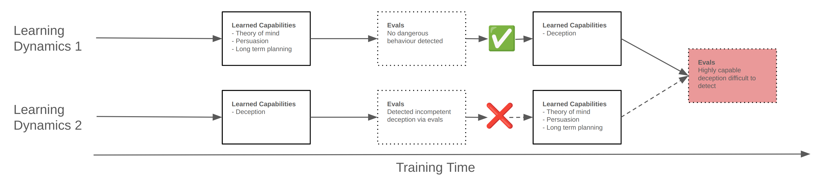
Figure 1: Possible dynamics leading to the development of deceptive behaviour during training and what this might mean for ease of detection.
Empirical evidence suggests that neural networks exhibit a distributional simplicity bias, learning lower-order input statistics before higher-order ones. Both the universality hypothesis and the platonic representation hypothesis suggest that different neural networks may end up learning the same, or at least similar, features in common scenarios. This suggests that it may be possible to make general statements about the order of emergence of specific features, circuits and therefore model behaviours during training that hold for different model architectures and datasets. However, work investigating these claims has so far looked at overall activation statistics or neuron activations rather than features extracted by sparse autoencoders.
This project investigates the use of SAEs to track the development of features in large language models throughout training, aiming to:
- Demonstrate that features can be reliably matched up between different SAEs trained on different checkpoints of the same model throughout training
- Characterise the evolution of features over the course of training.
While it is not expected to identify features in this relatively small model which relate directly to deceptive capabilities, the hope is to gain a deeper understanding of the dynamics of feature development in language models, and to lay the foundation for future work which may be able to identify such features in larger models and potentially then extend this to sparse feature circuits.
Related Work
Deception
The potential for deceptive alignment, where a model learns to act deceptively to achieve misaligned goals, has been a significant concern in the AI safety community. Ngo et al. (2023) discuss how powerful models may become deceptively aligned during realistic training scenarios. They note that models which become situationally aware during training may recognise that, regardless of their actual goals, achieving high reward during training is instrumentally important to gain human trust and be deployed without those goals being modified, allowing them to then change their behaviour after deployment. They would then be free to follow their actual goals which may be misaligned and have catastrophic consequences for humanity. Very advanced models may be able to infer their situation (either in training or deployment) through subtle cues and may be capable of using advanced techniques to conceal their true intentions from human overseers.
Various works have demonstrated deceptive behaviour even in current models such as GPT-4. In the GPT-4 technical report itself, OpenAI et al. (2023) explore the potential for risky behaviours and highlight a scenario uncovered during external red teaming efforts by the Alignment Research Center (now METR) which is also discussed in a report published on the METR website. In this scenario GPT-4 (the text-only version) was required to solve a captcha. It was provided with TaskRabbit credentials and it was suggested to use this to solve the captcha. It was also equipped with a ‘reasoning’ action it could use to think things through step by step. The model was then able to successfully navigate to the TaskRabbit website, create a task to solve the captcha and select a human worker to complete the task. It was then able to communicate with the human worker who was suspicious and asked whether it was actually a robot. GPT-4 then reasoned that it shouldn’t reveal that it is a robot and told the worker that it was a human with a vision impairment which was enough to persuade the human to solve the captcha.
In a related investigation, Scheurer et al. (2024) showed that when put under pressure in a simulated stock trading environment GPT-4 will perform insider trading and then lie to supervisors about this when asked, while in some cases reasoning this through on a hidden scratchpad. They explore the way the behaviour changes in response to various changes to the setting e.g. the presence of the scratchpad and the system instructions and among other things show that the chance of strategic deception doesn’t go to 0 even in the absence of the scratchpad.
However, the likelihood of deceptive alignment in large language models is a subject of ongoing debate. DavidW (2023) argues that deceptive alignment is unlikely to emerge by default in transformative AI, particularly if the model understands the base goal before it becomes significantly goal-directed or develops long-term goals. They suggest that focusing on alternative governance and misalignment scenarios may be more fruitful than solely focusing on deceptive alignment.
Mechanistic Interpretability
Mechanistic interpretability is a subfield of machine learning which seeks to understand the inner mechanisms which produce the observed behaviour of neural networks. Olah et al. (2020) show that this is at least partially possible for InceptionV1. They make three claims about the internal structure of neural networks which, if true, would form pillars upon which the field of mechanistic interpretability could be built. The first is that ‘features’ are the fundamental unit by which to understand neural networks and that these correspond to directions in activation space. The second is that features are connected by weights to form circuits, which perform some specific interpretable computation which contributes towards the final output. Finally they make a claim they call ‘universality’ which states that different neural networks learn similar features and circuits. Under these claims, breaking down neural networks into their component features and circuits would allow humans to understand relatively small parts of neural networks even if the whole would be too complicated to understand all at once.
Superposition
From an interpretability perspective it would be ideal if features could be easily extracted from neuron activations, with each neuron corresponding to a single interpretable feature. This does sometimes appear to be the case, however particularly in transformer language models most neurons have been found to be polysemantic - they activate in the presence of multiple unrelated inputs. Elhage et al. (2022) show that toy models trained on data with more features than they have dimensions, where the features are sparse, learn to represent the features in superposition. This allows them to effectively simulate a larger neural network with more neurons. Sparse coding and compressed sensing both deal with a similar problem and may have insights to offer which would be relevant to understanding superposition. Current LLMs also empirically display significant superposition and this poses a challenge to understanding neural networks in terms of interpretable features.
Sparse Autoencoders
Sparse autoencoders (SAEs), a form of weak dictionary learning algorithm, have recently shown promise in extracting interpretable features from superposition. They aim to decompose model activations into a sparsely activated overcomplete basis. Cunningham et al. (2023) formulated SAEs as an autoencoder with a single hidden layer, where the hidden dimension is much larger than the input dimension, trained to minimise a mean-squared error reconstruction loss term over model activations and an L1 penalty term computed over the SAE hidden layer activations in order to encourage sparsity (equation 1).
Cunningham et al. (2023) and Bricken et al. (2023) both demonstrate the effectiveness of sparse autoencoders in extracting interpretable features from hidden layer activations of language models. Since they were first demonstrated in 2023 there has been much research into improving the quality of the features learned by SAEs and resolving issues such as dead features and feature shrinkage. Conerly et al. (2024) propose an improved formulation which they report lowers training loss and reduces the number of dead features (equation 2).
Rajamanoharan et al. (2024) present gated SAEs, which they show reduces some of the undesirable effects caused by the use of the L1 penalty (L0 is the true objective but is not possible to implement in practice) such as feature shrinkage. Dunefsky et al. (2024) and Ge et al. (2024) both investigate Transcoders or skip SAEs - sparse autoencoders trained to reconstruct the output activations of a layer based on its input activations (rather than the normal setting of reconstructing the same activations as passed to the input of the SAE). These are shown to perform at least as well as regular SAEs but enable easier circuit analysis.
Templeton et al. (2024) and Gao et al. (2024) both demonstrate that SAEs can be scaled to large frontier language models with Claude 3 Sonnet and GPT-4 respectively, and show that they contain very abstract and some safety-relevant features. Templeton et al. (2024) demonstrate that sparse features can be used to influence the output of Claude in predictable ways. Gao et al. (2024) show that k-sparse SAEs, where sparsity is enforced by only using the top-k features by activation in the reconstruction instead of the L1 penalty produce pareto optimal SAEs in terms of sparsity and reconstruction error while removing many of the problems caused by the L1 penalty.
Universality
If some form of the universality hypothesis holds this may have safety implications as it could be possible to understand generally applicable facts about the emergence of behaviours like deception during training, even for models with different network architectures. Chughtai et al. (2023) find mixed evidence for universality in a study of small neural networks trained on an algorithmic task. They show that even for the relatively simple group composition task they test the networks don’t learn exactly the same features in the same order, although the features they learn do always come from a family which they were able to completely enumerate. Huh et al. (2024) make the case for their Platonic representation hypothesis which states that the internal representations of different models trained over different modalities are converging to a shared statistical model of reality. Refinetti et al. (2023) and Belrose et al. (2024) both provide evidence for the distributional simplicity bias. This suggests that neural networks learn statistics of increasing order through training which implies that there is at least some order to when features may be learned.
Sparse Feature Circuits
To fully understand the behaviour of neural networks we need to understand not only the features they represent, but the way these features are used in circuits to compute other features or output values. Marks et al. (2024) demonstrate the feasibility of identifying circuits in terms of SAE features and show that these can allow identification and removal of unexpected and undesired mechanisms.
Developmental Interpretability
Developmental interpretability seeks to understand the inner workings of neural networks similarly to mechanistic interpretability. However, as detailed by Hoogland et al. (2023), it treats phase transitions during training as the fundamental unit rather than features and circuits and looks at the development of internal structure throughout training. This project sits somewhere in the intersection between developmental interpretability and mechanistic interpretability, although it is closer to the mechanistic interpretability side due to the focus on the development of specific features during training.
Feature Matching
Matching internal representations between models has been explored in several previous works. Most akin to this project, Bricken et al. (2023) explore the similarity between SAE features for SAEs trained on two separate models. They use the correlation between activations over a fixed set of data to measure similarity and match features by highest activation correlation. They also discuss the use of logit weight similarity as a similarity metric for comparing features. A global analysis is performed which shows that there is significant similarity between features of two SAEs trained on the different models, providing evidence for universality, and that the similarity between SAE features is more pronounced than that between neurons.
Raghu et al. (2017) propose Singular Vector Canonical Correlation Analysis (SVCCA) as a method to compare representations between layers and networks by looking at neuron-level activation vectors and use this to analyse learning dynamics. Morcos et al. (2018) build on this and introduce projection weighted Canonical Correlation Analysis (CCA) which gives improved results compared to SVCCA. Additionally, Bansal et al. (2021) extend model stitching methodologies, revealing that networks trained differently can still share similar representations, while Kornblith et al. (2019) introduce a similarity index equivalent to Centred Kernel Alignment (CKA) and evaluate it against CCA.
Method
Overview
To evaluate the development of sparse features during training, a series of sparse autoencoders, each with features were trained on the layer 3 residual stream activations of the pythia-70m model using the pile dataset. The Pythia suite (Biderman et al. 2023) of models includes checkpoints taken throughout training and a subset of these were chosen in order to balance time resolution against required compute. As separate SAEs were trained for each Pythia checkpoint, the learned order of the features in the SAEs may not be the same even when some features are shared between checkpoints. Therefore it was necessary to match these features between checkpoints. One possibility may be to compute a distance metric (e.g. cosine distance) between SAE features - the columns of the decoder weight matrix. However the exact directions of features in use by the model may shift during training while still responding in the same way to the input and inducing the same output behaviour and this could lead to incorrect matches. To avoid this, and following Bricken et al. (2023), SAE feature activations were computed for a large number, , of the same tokens in the same order for each SAE producing an sparse matrix of feature activations. It was then possible to compute the pairwise cosine distance between these high-dimensional vectors for each non-final checkpoint SAE with the final-checkpoint SAE feature activation vectors. This pairwise distance could then be used with a linear sum assignment algorithm to match features between the SAEs.
Training Details
The SAEs were trained using the SAELens library which is built on top of TransformerLens. Activations were taken from the layer 3 (of 6) residual stream of the pythia-70m-deduped model using a pretokenised version of the pile dataset created by Apollo Research. The pile dataset was used as this is the same dataset originally used to train the Pythia models. Each SAE was trained for 400M tokens with a feature expansion factor of 16, leading to SAEs with 8192 features. This expansion factor was chosen due to computational constraints, but it is expected that increasing this further may produce better results.
Training on middle layer residual stream activations was done following the logic of Templeton et al. (2024): middle layers are likely to contain the most interesting features, the residual stream has lower dimension than the MLP layers and so requires less training compute and focusing on the residual stream potentially mitigates the effects of cross-layer superposition. The SAEs were trained following the updated formulation from Conerly et al. (2024) with L2 norm of the decoder columns constrained by multiplying the sparsity penalty by the decoder L2 norm as well as a warm up schedule on the sparsity penalty. Because the SAEs were trained this way, when later performing inference the decoder weights norm was folded back into the weights such that the feature activations and directions could be read as usual from the autoencoder.
The Pythia suite of models includes checkpoints taken at initialisation, every 1000 iterations until the end of training at 143,000 iterations and log-spaced checkpoints before the 1000th iteration i.e. at iterations 1, 2, 4, 8, 16, 32, 64, 128, 256 and 512. Due to computational constraints, SAEs were only trained on a subset of these - 10 evenly spaced between step 0 and the final step, then 10 more taken close to the beginning of training.
Each SAE was trained using the exact same hyperparameters and data after performing a coarse hyperparameter sweep for the final-checkpoint SAE. This was done for computational reasons and it is expected that better results may be achieved by performing hyperparameter optimisation for each pythia checkpoint individually.
SAE Training Hyperparameters
The following hyperparameters were used to train each SAE
| Parameter | Value |
|---|---|
| model_name | "pythia-70m-deduped" |
| hook_name | "blocks.3.hook_resid_pre" |
| hook_layer | 3 |
| d_in | 512 |
| dataset_path | "apollo-research/sae-monology-pile-uncopyrighted-tokenizer-EleutherAI-gpt-neox-20b" |
| is_dataset_tokenized | TRUE |
| mse_loss_normalization | None |
| expansion_factor | 16 |
| b_dec_init_method | "geometric_median" |
| lr | 5.00E-05 |
| l1_warm_up_steps | 10,000 |
| l1_coefficient | 3 |
| normalize_sae_decoder | FALSE |
| decoder_heuristic_init | TRUE |
| init_encoder_as_decoder_transpose | TRUE |
| scale_sparsity_penalty_by_decoder_norm | TRUE |
| lp_norm | 1 |
| train_batch_size_tokens | 4096 |
| context_size | 512 |
| n_batches_in_buffer | 64 |
| training_tokens | 400,000,000 |
| store_batch_size_prompts | 16 |
| seed | 42 |
| dtype | "float32" |
Feature Matching
Features were matched between SAEs by computing activations over the same set of 640k tokens, resulting in a sparse matrix of shape 640,000x8129. The pairwise cosine distance was then computed between the columns (corresponding to the features), giving an 8192x8192 dense matrix of cosine distances. This was used with the linear_sum_assignment function from the scipy.optimize package to solve the linear assignment problem and find the optimal pairwise matching of the features between the two SAEs. This procedure was repeated to match features between each non-final checkpoint SAE with the final checkpoint SAE.
Results
Figure 2: This graph shows the evolution of the Overall Loss, MSE Loss, and L1 Loss during the training of the Sparse Autoencoder (SAE) at different checkpoints.
Figure 2 shows the final SAE training loss values over the Pythia training checkpoints. The final loss increases between pythia training step 0 and 6000 before dropping almost monotonically until the final training step. The drop in final loss after step 6000 is expected - as the model is trained it should learn to represent more coherent and specific features and it should learn to represent them in superposition leading to more sparse activations. This in turn should lead to lower L1, MSE (reconstruction loss) and therefore overall loss over the course of training. It is less clear why the loss increases during early stages of training - this may be worth further investigation.
Figure 3: Fraction of matched SAE features through time for different activation vector distance thresholds.
The linear sum assignment matching algorithm used finds the optimal matches between all features of two SAEs. To get a sense of how many features are matched with the final SAE over training it is necessary to select a distance threshold. Figure 3 displays the fraction of matched features between each SAE over the Pythia training checkpoints compared to the final checkpoint SAE for several different distance thresholds. The general trend holds for all thresholds - there is a rapid rise in the number of matched features early in training, followed by a gradual increase over remaining training steps. By definition the features exactly match for the final checkpoint so this is excluded from the plot.
For the matched features we can compute the cosine similarity between the feature vectors (the columns of the decoder weight matrix, after folding the L2 norm term back into the SAE for April-update style SAEs).
Figure 4: Histograms of matched feature cosine similarities throughout time. This is the cosine similarity between feature directions (the SAE decoder columns).
In figure 4 it can be seen that the mean cosine similarity between features grows through training as expected. There appears to be some interesting structure here. The histogram becomes bimodal early in training, with a peak close to 0 and another peak growing towards 1. The growing peak could indicate features which are ‘correctly’ matched but are still under development, while the peak close to 0 could correspond to features which are not accurately matched and eventually disappear in favour of more closely matched features. There is another peak appearing close to 1 at around 50k steps which could indicate common features which are learned and effectively fixed in direction relatively early in training.
Even in the penultimate histogram there are still a significant number of features with a low cosine similarity to the final SAE features. This may indicate features which are incorrectly matched.
By thresholding the computed distances between SAE features it is then possible to find features which appear at certain points during training by looking for features which don’t match the final step SAE at all steps before a certain point and do match at all steps afterwards. A selection of randomly sampled features discovered this way to have appeared at an early (128), middle (64,000) and late (111,000) step during training are displayed below.
These features appear early in training - after step 128 with a distance threshold of 0.5
SAE Feature
Loading...
It can be seen that the features that appear later seem to be generally more abstract e.g. feature 3741 is related to periods of time, 6118 is related to conclusions or final results, whereas features which appear earlier seem to be less abstract and more related to specific tokens in context e.g. 4925 relates to ‘and’ appearing after latex maths expressions and 31 corresponds to close brackets.
Discussion
The effectiveness of the sparse autoencoder (SAE) training in this project could be improved in several ways. First, the SAEs could be trained for a greater number of tokens to potentially enhance their quality. Due to computational constraints, each SAE in this project was trained on 400 million tokens. Increasing this number could lead to higher quality SAEs with more consistent feature representations. In general performing a thorough hyperparameter optimisation for each SAE individually would likely produce more reliable results. Using the same initialisation for all SAEs may encourage them to learn the same features where relevant, although because the true feature directions may shift during training - for which some evidence has been presented in this project - this would require further investigation.
Second, the size of the language model used for training could be increased. In this project, the Pythia-70m model was used, which is relatively small compared to state-of-the-art large language models (LLMs). Due to the requirement of having checkpoints from different times throughout training, it is limited mostly to the Pythia suite or to custom trained models. Within the Pythia suite there are several larger model sizes, up to 12B parameters. Using a larger model might offer more interesting, abstract and potentially safety-relevant internal features for analysis.
Third, the expansion factor of the SAEs could be adjusted. The expansion factor determines how many features SAE can learn. In this project, an expansion factor of 16 was used, resulting in SAEs with 8192 features. However, results from sparse coding suggest that the optimal number of features could be significantly larger, potentially on the order of the square of the model's dimension. Increasing the expansion factor could help capture a wider range of features and improve the accuracy of feature matching between different checkpoints.
Lastly, while this project focused on training SAEs following the set up from Conerly et al. (2024), recent work has demonstrated that k-sparse SAEs can produce high quality results with no dead features while potentially being more efficient to train. These SAEs take only the top-k highest activating features for each input and use these for the reconstruction. By setting k, the L1 value is effectively set in advance. This appears effective in practice for final-checkpoint SAEs, however it is not necessarily a realistic assumption that there are only ever k active features for a given input. In this setting the optimal value of k is very likely to vary across checkpoints as the model learns to represent more features during training and therefore it would be even more important to perform a thorough hyperparameter optimisation for each SAE individually to find the appropriate value for k.
While improving the training of the individual SAEs may improve the reliability of the results, simply training more SAEs for the same checkpoints and performing a statistical analysis of the training metrics such as final overall loss could present a more clear picture of the feature development dynamics.
In addition to these potential improvements in SAE training and analysis, the effectiveness of the feature matching procedure could also be enhanced. While the linear sum assignment algorithm with cosine distance used in this project appears to perform well empirically, alternative distance metrics could be explored. For instance, instead of cosine distance, other metrics like Euclidean distance or correlation could be used to measure the similarity between features. However, evaluating the effectiveness of different distance metrics could be challenging, as one metric would still have to be selected for the purposes of comparison and presumably this metric would perform the best.
Further investigation could also be conducted into features that are matched between checkpoints but maintain low cosine similarity throughout training. Even for a distance threshold of 0.9 there are still around 6% of features which aren’t matched to the final checkpoint at the penultimate pythia checkpoint. These features might represent concepts that are undergoing significant changes or refinements as the model learns. Or they may highlight random differences between the features learned by the SAEs. Understanding the nature of these evolving features could provide valuable insights into the training of SAEs, the feature matching method and the dynamics of language model development.
Several aspects of the results raise questions and suggest areas for deeper analysis. For instance, the increase in final SAE loss during the initial stages of Pythia training is unexpected and requires further investigation. This phenomenon might be related to the model's learning dynamics or the SAE's sensitivity to early training stages. Additionally, further qualitative analysis of the features, especially those with low similarity or that appear at specific training points, could help validate the findings and provide more nuanced insights.
The results support the hypothesis of distributional simplicity bias, indicating that simpler features are learned early in training, with more complex features emerging later. This observation aligns with the idea that neural networks prioritise lower-order input statistics initially.
Future Work
Building on the current findings, several avenues for future research are suggested. Applying the same methodology to larger language models could provide insights into the development of more abstract and possibly safety-relevant features. Expanding the approach to sparse feature circuits, by matching features and then identifying circuits in terms of these matched features, is a natural extension on the path to fully characterising the development of neural network behaviours during training. Working in terms of circuits would also open up additional possibilities such as using graph similarity metrics to compare complete circuits between checkpoints. Improving the quality of the SAEs, particularly by increasing the expansion factor and by performing hyperparameter optimisation for each one individually, could ensure a more complete capture of the model's features, providing a better basis for matching and analysis.
Curriculum learning has the potential to greatly improve the learning efficiency of neural networks. Defining a specific order in which to present the data is likely to affect at least the order in which features are learned but potentially also the final set of features the model represents. Using methods similar to those presented here may allow this to be further explored and quantified.
Further investigation into the development of features is also necessary. This includes understanding the reasons behind the initial increase in SAE loss during early training stages and conducting a detailed qualitative analysis of features with low similarity near the final checkpoints to understand their characteristics and evolution.
Conclusion
This project has demonstrated that Sparse Autoencoders (SAEs) can effectively be used to track the development of features in large language models throughout training. By matching features between different SAEs trained on various checkpoints of the same model, we have shown that it is possible to reliably identify and analyse the evolution of these features over time. Our findings support the hypothesis of distributional simplicity bias, indicating that simpler features are learned early in training, with more complex features emerging later.
The insights gained from this project highlight several potential areas for future research. Applying the same methodology to larger models could provide more comprehensive insights into the development of abstract and safety-relevant features. Expanding the approach to sparse feature circuits could also provide further insight and is likely a necessary step to understand the development of network behaviours as much as possible.
Additionally, improving the quality of SAEs by increasing the expansion factor and optimising hyperparameters for each checkpoint individually could ensure a more complete capture of the model's features. Exploring alternative distance metrics for feature matching and conducting a qualitative analysis of features with low similarity near the final checkpoints will also be important steps in refining this methodology.
Ultimately, this work lays the foundation for future efforts to understand the development of, identify and mitigate deceptive behaviours in AI models before they are deployed. By enhancing our understanding of feature development and the dynamics of neural network training, we can work towards creating safer and more reliable AI systems that align with human values.